I vaguely recalled early in my finance education that among the first topics covered was “risk”. And typically, volatility is often brought up as a key risk metric. When I first learned about risk and volatility, I took it for granted that the higher the volatility, the riskier an investment would be. It’s easy, it makes sense at first thought, and it’s convenient. And many thought the same.
As I gradually got more exposed to the world of derivatives and quantitative finance, more questions came. Risk is no longer that straightforward, and often contextual — the concept and measure of risk vary in different situations. As part of the Quant Simplified series, I hope to share more about risk and volatility and discuss the various context that gives risk a different meaning.
A quick recap — risk and volatility
Volatility, by definition, is a statistical measure of the dispersion of returns for a given asset. Mathematically, it’s referred to as the standard deviation σ and some may refer to the variance of the returns. Consider the daily return on an asset to be r, the daily return volatility follows the same equation as getting the standard deviation of the daily returns, as follows.

One thing to note is that more often than not volatility is quoted as annualized. The annualized daily return volatility would simply be the daily return volatility multiplied by the square root of the number of trading days in a year. Usually, one would assume 252 trading days per year for simplicity.
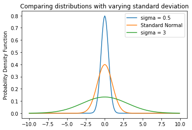
Volatility is an intuitive measure of risk; the higher the volatility, the higher the dispersion of the asset prices. As Figure 1 shows, the greater the volatility, the wider the range of the asset's daily returns. The more uncertain the price is, the greater the risk. So far so good.

How does one interpret volatility? What does a 1.2% (non-annualized)12-month daily return on the DAX index mean intuitively? If one were to make an assumption that the daily return follows a normal distribution, this would mean that over the past 12 months, 68% of the time the daily return falls within +/- 1.2%. This is a simple application of the 68–95–99.7 rule.
However, it is important for one to be mindful that the 68–95–99.7 rule at best is a rough (and naive) estimate of the return profile. This is because asset return does not necessarily follow a normal distribution.
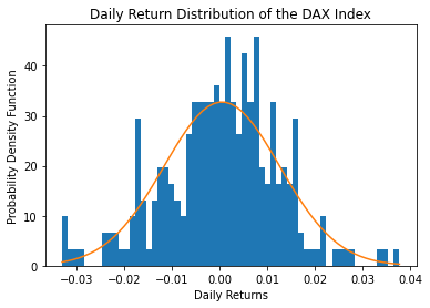
As observed empirically, drastic price movements do happen especially when there are risk events happening at the backdrop. This creates a “fat-tailedness” in the distribution, in which extreme ends of the distribution have a higher probability density than that of a normal distribution. In addition, there are more often negative price movements than there are positive price movements. This led to a skew in the distribution. Figure 2 illustrates the non-normality of returns perfectly. The DAX index has fat tails (excess kurtosis of 0.48) and a negative skew (-0.17).

Nevertheless, the normal assumption is convenient and often not too wrong. Using the rule would help laymen grasp the concept easily as well.
Portfolio performance — risk and return
One application of volatility is to quantify a portfolio's performance. A portfolio is a collection of tradable assets — across different asset classes in the form of various instruments — held for the purpose of investing. One can either manage one’s own portfolio by trading the assets directly or by taking a share of other’s portfolios and seconding the risk management work to the portfolio managers. The latter comes in the form of fund products, such as exchange-traded funds, mutual funds, or, for accredited investors, hedge funds.
When investing in passive funds, the expectation of the fund's performance is that it tracks the benchmark index that it supposedly follows. Thus there is no expectation for it to outperform the benchmark, and the cost is lower. On the other hand, for actively managed funds, a high premium is paid for management fees. Therefore, there is a need to compare two different funds to determine which performs better and at a reasonable premium.
Comparing average returns is not sufficient most of the time. For two funds with the same average returns, would one prefer the fund with less volatility over the assessment period or the one with more volatility? How much more volatility would one be willing to accept for a fund with a higher mean return? Thankfully, one widely accepted and used portfolio metric is the Sharpe ratio. It takes into account volatility and average return in the assessment of portfolio performance. Loosely interpreted, it is the measure of the excess return of the portfolio (over the benchmark) per unit of risk taken. Intuitively, the higher the Sharpe ratio, the higher the additional return made above the benchmark, rebased on the volatility of the portfolio's excess return.

A commonly used benchmark is the risk-free rate of return. If another benchmark is used, some may refer to this as the information ratio instead.
Risk and Psychology
Well, all is good thus far with measuring risk. However, some might immediately see a small problem with volatility as a measure of risk. Mathematically, ‘risk’ simply refers to the uncertainty of asset return, but does not put different weights on positive deviation and negative deviation. ‘Risk’, in reality, tends to have a negative connotation among people. People love positive returns and hate going into negative. There ought to be some differentiation, ain’t it?
Indeed, the Sharpe ratio does not take into account the psychological interpretation of ‘risk’. Some may use skewness as a rudimentary measure to account for this, but skewness — along with other higher moments of distribution — is mathematically rigorous to compute and not as intuitive to the masses. We ought to introduce something simpler.
One candidate that is widely used in portfolio management is the Maximum Drawdown (MDD). Unlike volatility, MDD is rather simple mathematically. It measures the largest price drop from a peak to a trough over a given period of time. Measured in percentage terms, it gives one a good idea of how much one would lose if one were to enter the position at a peak. Figure 3 illustrates how MDD is calculated on the DAX Index.

Another candidate to measure downside risk is the Sortino ratio. The Sortino ratio looks very similar to the Sharpe ratio, with a slight tweak in the denominator. Instead of using the volatility, the semi-deviation of the return is used.

Semi-deviation differs from standard deviation in that only negative deviations are taken into account, and all positive deviations were given a zero weight. As such, all positive price deviations were ignored, and only the negative price deviations were included in the risk measure.
Risk and Regulation
Apart from measuring portfolio performance, ‘risk’ is a huge regulatory topic. Following various market events from 1992 that led to huge losses in the international markets, the Basel II Accord was introduced. The Accord mandates financial institutions to use standard measurements for credit, operational, and market risks. For market risks specifically, it was stated that the Value-at-Risk (VaR) approach is much preferred.
The VaR is a statistical measure of the riskiness of a portfolio of assets, which gives the maximum dollar amount expected to be lost over a given time horizon. This can be used on a portfolio level or a firm level to assess potential losses. It requires 2 key parameters, namely the significance level (α), and the risk horizon.
The Basel II Accord requires a 1% significance level in VaR calculation, i.e. to calculate a 99% VaR. Consider a firm with an average Profit-and-Loss (PnL) of $66,000 and volatility of $100,000. Figure 4 shows the cut-off point of the 1% significance level on the Profit-and-Loss distribution. The 99% VaR of this firm is $166,635. Loosely interpreted, we say that the firm has less than a 1% chance of losing more than $166,635.

The calculation of VaR is often not an easy topic and may require the use of simulation tools such as the Monte-Carlo simulation. More details of VaR calculation may be covered in future chapters. As a beginning, knowing VaR exists and what it means is important at the beginning of a quant’s journey.
Risk — looking back or looking forward?
In the large part of this chapter, we have looked in depth volatility as a measure of risk. However, the volatility used is based on historical data, and the purpose of risk measurement here is for reporting. Would historical volatility be useful as a measure of the current (and future) risk of the asset? If not, what would be an alternative?
Ideally, we’d want to know the current risk of investing in an asset. However, historical volatility does not equal actual volatility. While there are models that allow one to predict future volatility, predictions are simply educated bets and there is no guarantee that the prediction will always converge to the actual volatility.
Thankfully, though we may not be able to tell what is the actual volatility, we can get a feel of what the market thinks the volatility would be. This relates to the options market, where one can derive the implied volatility from the option prices.
Options, one of the commonly known derivatives, give the buyer the right, but not the obligation, to fulfill the contract. A call (put) option gives buyers the optionality to purchase (sell) an underlying asset at a predetermined (aka strike) price at a future date. Due to their properties, options are an effective tool for hedging and speculating.
Options are generally priced using the Black-Scholes equation, which takes in the strike price, volatility, interest rate, time-to-expiry, and current underlying asset price (aka spot price) to generate the value of the option today.
Generally, out-of-the-money (OTM) options (where the potential payoff is zero) are cheaper. The deeper in-the-money (ITM) an option is, the more expensive it gets. Thus, most trading occurs on at-the-money (ATM) or OTM strikes. And the market price of the options would increase when there is more demand to get into an option position.
Like how one can derive an option price with a given volatility, the reverse is the same. And most of the time, the volatility is unknown, but market prices — driven by the forces of demand and supply — are known. By working to solve the Black-Scholes equation backward, one can then get the “implied volatility” of the option for a given market price. This gives us an indication of how much is the market “pricing the volatility”. The higher the implied volatility, the higher the perceived risk.
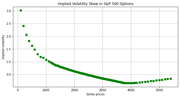
Implied volatility is not static across all strike prices. Figure 5 shows a typical implied volatility profile of OTM/ ATM index options. Index options tend to exhibit a “skew/smile”, where implied volatilities are higher at one end compared to the other, with a minimum somewhere in near at-the-money strike. The higher implied volatilities at extreme ends are due to higher trading activities on the OTM strikes (due to the options being cheaper). Significantly higher implied volatilities are observed at lower strikes due to the need for downside protection. Investors enter OTM put options (lower strike range) to hedge a potentially large downside price movement. Thus, the higher the OTM put option implied volatility is, the more fearful investors are.

Now that we have linked implied volatilities to a fear gauge, this brings us to a new asset class — the volatility asset. Because implied volatilities are derived from tradable options, we are able to construct an index that gives one an indication of what the market thinks of the current volatility. This is the essence of volatility indices such as the VSTOXX index (based on EURO STOXX 50 options) and the VIX index (based on S&P 500 options). Both indices offer a glimpse of the implied variance/ volatilities priced into the respective option markets, thus showing the extent of investors’ confidence.
With an index, one is able to trade the derivatives on implied volatilities. The VIX futures and VSTOXX futures allows one to hedge or speculate the forward implied volatilities of the market. Details of the volatility index and derivatives shall be covered in future chapters.
All in all, we have covered risk and volatility to a good extent in this chapter — from the basic understanding of volatility, the various risk metrics that rely upon historical volatility calculation, the limitations of volatility as a risk measurement in portfolio management, and implied volatility as an indication of market perceived level of risk. This chapter also offers one a good glimpse of various topics in quantitative finance and a simple explanation of key terms.
I hope you enjoyed this article, and find this a useful primer (for the unacquainted) or summary (for the well-informed). Do comment with your feedback to help improve the series, and let me know what you’d like to see for future chapters. Thanks for reading!
